Implementing & Using Low Density Parity Check Codes

Low density parity check codes using irregular graphs show promise for high error correction rates with linear time and space requirements, but as of yet there has not been an analytical way to find precisely, or even approximately, which classes of irregular graphs produce good error correction rates. We have implemented a portable, versatile toolkit for using and testing different parameters to LDPC codes. This paper contains instructions for interfacing with the code as well as specific implementation details. In this implementation, encoding and decoding have time and memory requirements linear in the number of edges. We implement two forms of decoding, referred to as hard decision decoding and belief propagation decoding. While the belief propagation algorithm gets consistently higher error rates than the hard decision method, it does so at the expense of additional time and space needed for floating point calculations. In certain situations, sacrificing error correction rate for the speed of hard decision decoding would be useful. Preliminary testing of the coding package using belief propagation indicates that it achieves error correction rates comparable to those in Luby's[3] original paper.

1 Introduction

The recent rise of wireless electronic devices has generated practical interest in the field of error correction. With wireless networks prone to introducing errors in transmission, researchers have focused on developing and refining encoding schemes that add redundancy to transmitted data in order to recover errors.

In the past few years, researchers have reexamined work by Gallager[1] on low density parity check codes using regular graphs, which give good high correction rates and good speed and memory requirements. Luby et al.[3] extended this idea to use irregular graphs to get higher error correction rates. Their motivation was that regular graphs with low degree have better performance. However, nodes of high degree correct their value more quickly, so using irregular graphs could mitigate those two opposing characteristics. Currently unknown are exactly which families of graphs behave well for these codes; Luby's paper uses edge frequency distributions that work well for Tornado codes, a similar-looking erasure code developed by his research group[2]. As of now, no analytical method for choosing good graphs exists. Therefore, the trial and error mechanism is the best route for finding graphs with good error correcting properties.

We provide a toolkit with the main motivation to provide researchers with the framework to evaluate and improve upon the codes, making it easy to test various graphs with different size data inputs. This framework supports regular and irregular graphs, along with hard decision and belief propagation decoding. It includes automatic support for the binary symmetric channel along with framework for the user to add information about his/her specific Gaussian channel.

In addition, we include a command-line utility for testing the codes using the belief propagation algorithm and the zero data set, allowing for variations in graph descriptions, code rates, and graph sizes to quickly test the performance of a given graph description. Preliminary results indicate that, when using the same codes as presented in the Luby paper, our implementation of the codes yields comparable error correction rates. This code base could be used as a framework for research to find graph descriptions that correct error rates nearer to the Shannon limit than those presented in the Luby paper.

The rest of this paper is outlined as follows: Section 2 discusses the high-level objectives in LDPC implementation, and Section 3 describes how one would interface with the C++ code to try out various graph descriptions or to use the program to encode and decode a data set. Section 4 discusses specific details about data representation and algorithm implementation, and Section 5 gives preliminary performance numbers, indicating error correction rates and time and memory usage. Finally, Section 6 discusses extensions that could be made to this code base to improve its performance.

2 Design Goals

Our code design had three driving design goals: portability, a simple interface, and efficiency. Portability is key, because the decoding machine should not need any specific knowledge of the machine used to encode the message. Because the codes rely on graphs, graph construction must be done in a systematic way such that both ends build the same graph. One component of portability is the pseudo-random number generator, which must be included with the LDPC code suite in order to remove machine dependencies on random number generators. Another consideration of portability is to make certain that any rounding that ever occurs happens in a consistent and predictable way. This comes into play most visibly when translating frequencies of nodes or edges to actual numbers when building the graph. See Section 4.3 for more information on the remedy to this problem. To keep the interface clean and simple, we encapsulate all functionality in a single C++ class which supports multiple graph descriptor formats. The enclosed test suite provides logical entry points to the code base to make it easy to try out the coding process, even without fully understanding the algorithm. Finally, the coding process needed to be as efficient as possible. The algorithm can be implemented a number of ways, but there exist implementations which have speed and memory usage linear in the number of edges. One consequence of this characteristic is that the graph representation is specialized for coding. We are creating a coding package, not a graph package. So, most likely, the graphs used here will not be useful in other contexts.

We anticipate two main target audiences for this implementation: researchers and evaluators. The research audience would be those trying to find and test different graph descriptions to find graph families that give high error correction rates, most likely those trying to find ways of approaching the Shannon limit. This implementation puts in place the framework for such testing. The other potential audience is those we refer to as evaluators, who are people who wish to evaluate the performance and/or feasibility of LDPC codes for possible use in a real (i.e. non-research) setting but do not want to use the resources for their own implementation of a code that they may not even end up using. This code base and testing framework allows for straightforward feasibility studies.

3 User Guide

3.1 Using the decode test program

We provide a simple command line utility called decode for testing belief propagation decoding. It allows full control over the following parameters:

3.2 LDPC class description

All the functionality for the low-density parity check codes in encapsulated in a single C++ class. Different versions of the constructor take different graph specifications to allow the user to specify node degree frequencies, edge degree frequencies, or node degree counts to describe the graph family. To specify the specific graph, the user can input either the number of data nodes and a code rate or the number of data nodes and number of check nodes. In addition, the constructor needs a PRNG seed, presumably the same one used on both the encoding and decoding ends.

The encoding and decoding processes are methods of the class. Encoding is a straightforward process that requires construction of a graph and a simple computation of the right node checksums. The class provides several decode methods, implementing both hard decision and belief propagation decoding. Each decoding algorithm provides for decoding with reliably transmitted check nodes and decoding where the right nodes are assumed to be all zero. In addition, the belief propagation decoder has support for Gaussian channel input. More detail on this is found in Section 4.7.

In addition, we provide utility functions for converting between different graph family specifications without needing to invoke a graph constructor. See Section 4.3 for more details.

4 Implementation Details

4.1 Data representations and assumptions

We represent a graph by a list of edges, sorted by left node. All edges for a given node appear adjacent in the edge list; in fact, the edge data itself includes only the right node identifier. The left node is implicit; whenever we reach a new left node on the list, the NEW_NODE_FLAG of the edge is set, so it is simple to keep a counter of which left node we're on when passing through the edges sequentially.

We assume that the PRNG seed and right nodes are transmitted reliably. Without a reliable PRNG seed, the decoder would not build the same graph as the encoder, and decoding would fail. The reliable right side is necessary because our decoding algorithm corrects errors in left nodes based on disagreements with right node checksums. This reliable transmission on the right can be accomplished with cascading LDPC encodings or with a Reed-Solomon code. In addition, we allow for the special case in which all right nodes are zero. This can occur when testing for error correction rates of a specific graph by simply using the zero data set, or the user can arrange the graph such that all right nodes are forced to zero.

4.2 Pseudo Random Number Generator

We supply a simple linear congruential pseudo-random number generator so that both the encoder and decoder build the same graph. We chose this family of PRNGs because of its speed, which is essential when so much randomness is needed for building these irregular graphs. Our current PRNG, which can easily be replaced by the user, is $y_{n+1}=69069y_{n}+1 (\hbox {mod} 2^{32})$ , where $y_{0}$ is simply the seed required by the graph constructor[5]. Because this PRNG behaves deterministically, the encoder and decoder will work from identical graphs.

4.3 Graph representation conversions

Converting from node degree frequencies or edge degree frequencies to node degree counts, which is the representation actually used to construct the graph, happens systematically in the attempt to avoid problems in rounding across different machines and operating systems. Conceptually, node frequencies are represented by a set of ordered pairs $(d_{i},f_{i})$ , where $d$ represents the degree of the node, and $f$ represents the percentage of all nodes which have degree $d$ . There are $n$ such ordered pairs, with the stipulation that $\sum f_{i}=1$ . To compute the actual number of left (or right-the process is identical) nodes which have degree $d_{j}$ , first compute the cumulative frequency, given by

Also keep a running total $N$ of the number of nodes assigned thus far. Then the number of nodes of degree $d_{j}$ is equivalent to $F*(\hbox {total left nodes})-N$ . This round-as-you-go approach reduces the possibility that multiple rounding errors will add up and cause the graph to have too many nodes of degree $d_{n}$ . All conversions to node counts come from node frequencies; therefore, if the user inputs edge degree frequencies, those are first converted to node degree frequencies and then to node counts.

In addition, the conversions have built in provisions to ensure that the total number of edges coming out of the left side of the graph is equal to the number of edges going into the right side of the graph. Generally, rounding errors are such that both sides of the graph do not come up with the same number of edges. The converter uses the convention that the number of edges going into the right side as the correct number of edges. If the left hand side has $e$ extra edges, then $e$ of the edges of degree $d_{n}$ become edges of degree $d_{n}-1$ , which often involves introducing a new degree of edges. Additional details occur if $e$ is greater than the number of nodes of degree $d_{n}$ . This process occurs rarely and is described in the code comments. If the left hand side has $e$ edges too few, then the opposite happens. Those $e$ edges become edges of degree $d_{n}+1$ . We work on the assumption that by making the changes in degree to those nodes of the largest degree, we will have a smaller overall impact on the behavior of the graph.

4.4 Graph construction

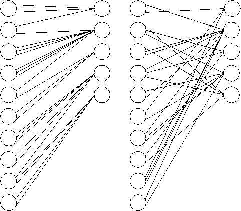
The graph constructor takes a list of node degree counts as input and creates the graph in three steps. In the first step, the node degrees are randomly assigned and the edges are given an initial layout. The constructor steps through the nodes sequentially from top to bottom on both sides at the same time. As it encounters each new node, it picks a random index into the list of remaining node degrees for the appropriate side. The process is analogous to drawing the node degrees one at a time from a hat and assigning them to nodes. As each node degree is selected, the constructor places the appropriate number of edges in place, and this is how the degree is remembered. The left side of Figure 1 shows a graph after this process has been completed.

The second part of the process is to permute the edges. The edge list is swept from beginning to end, and for each edge location (which implies the adjacent left node) a random edge is chosen from the remaining edges (forward in the list). Effectively, the right side of the edge is drawn from the remaining possible right side locations and assigned to the current left node. When this process is complete, the edges are randomly assigned as illustrated in the second part of Figure 1.

**Figure 1:** Graph construction occurs in three phases. The first, shown on the left, assigns edges sequentially to create the desired node degrees on each side of the graph. In the second phase, shown on the right, the constructor randomly swaps edges to nearly complete the construction. In phase three, not pictured, we swap duplicate edges.
$\includegraphics{construct}$

This process leaves the possibility of duplicate edges and other small cycles. In the third part of the graph construction process, we remove duplicate edges. Each left node is scanned sequentially for duplicate edges. When one is found, it is randomly swapped with another edge in the graph (again, this has the effect of swapping the right side of the edge), making sure that the swap does not itself create another duplicate edge for either involved node.

This graph construction algorithm has a few advantages. The graph is created with the precise number of nodes of each degree as specified by the user, so experiments with different node degrees will not be skewed by random variations in the graph construction. Conceptually, the node degrees are laid out randomly and then the edges are distributed randomly into the available slots; we do not have to trade any randomness in edge placement to get precise control over node degrees. All computations are done with integers so there is no danger of rounding errors varying on different platforms, which is critical for the graph constructor. Since we also provide a pseudo-random number generator, graph construction is completely deterministic for a given set of input parameters.

4.5 Encoding

Encoding is straightforward and is done in a single pass through the edge list once the graph has been constructed. The right nodes are initially set to zero. Then, for each edge in the list, the current right node value is summed modulo two with its corresponding left node value.

4.6 Hard Decision Decoding

In hard decision decoding, each right node casts a vote to each of its adjacent left nodes as to what value that left hand bit should have. Each vote is determined by summing the adjacent left nodes modulo two and comparing the result with the check node that was computed at the time of encoding. In our implementation, we start each round of voting by initializing the right nodes to the check node values and then adding the adjacent left nodes modulo two (much like the encoding process). For a correct set of left nodes, the result is all zeros on the right side. Each node with value one on the right side means that that node votes for each of its adjacent left nodes to change its current value (since this would force the right node to zero). To actually tally the votes, the decoder iterates through the edge list a single time. The adjacent edges for each left node appear together, so it is convenient to collect the votes from all the adjacent right nodes, and the result is checked to see if the vote is decisive as determined by the voting thresholds that the user specifies for each iteration. If the voting is not decisive, then the left node is restored to its transmitted value.

In all, each iteration of the algorithm requires two passes through the edge list. The decoder completes successfully when all of the right nodes agree with the original check nodes. It this does not happen after a specified number of rounds, then the decoder terminates in failure.

Hard decision decoding does not give error correction rates as high as the belief propagation method. Even for irregular graphs, the highest rate of error correction Luby et al.[3] obtained was 6.27%. However, that does not negate the usefulness of this method in certain situations. For example, in a channel with small error rates, for example, 5% or less, in which decoding speed is a primary consideration, hard decision decoding would perform admirably. It uses integer and bit operations and is a good candidate for hardware implementation. This method sacrifices some error correction in order to achieve greater speed.

4.7 Belief Propagation Decoding

Using the algorithm described by MacKay[4], belief propagation decoding proceeds in rounds, each round updating a pair of variables associated with each edge. One variable, denoted by $q_{ml}$ , represents the probability that left node $l$ has a value of $0$ given the information gathered from all the check nodes other than $m$ . The other variable, $r_{ml}$ , indicates the probability that the right node $m$ is satisfied given that the left node $l$ has fixed value $0$ and including information obtained from other edges leading into node $m$ . Decoding proceeds in two passes per round, updating the $q$ variables in one pass and the $r$ variables in the other pass. Each round, the left nodes are tentatively assigned values of $0$ or $1$ based on the information gathered from all $q_{ml}$ for each data node $l$ , treating the values obtained as probabilities that the left node is $0$ and rounding appropriately. The algorithm terminates when a tentative assignment satisfies all the check nodes. If the algorithm does not terminate with success after a user-specified number of rounds, the decoder terminates with failure.

Currently, the belief propagation decoding algorithm supports input from the binary symmetric channel, requiring the error fraction of the channel to compute initial probabilities to start decoding. The framework is in place to support decoding from the Gaussian channel; only initial probabilities change. However, the exact values of the initial probabilities are dependent on the specific Gaussian channel, and so a user wanting to decode over the Gaussian channel must first normalize the values obtained from the channel to be probabilities.

In empirical trials, belief propagation easily outperforms the highest error correction rate for hard decision decoding cited by Luby. However, it does so by using floating point calculations, storing the large variables and performing the expensive arithmetic operations. As a result, in practice such high error correction rates would be relatively slow, although still linear time.

5 Performance

5.1 Speed/Memory usage

The graph representation and decoding algorithms are constructed in such a way as to keep the amount of time and space linear in the number of edges. As evident in Table 1, both time and memory usage increase linearly with the number of data bits. Therefore, splitting up a large message into smaller pieces, encoding and decoding each one separately, would not speed up the overall process. However, if only a fixed amount of memory is available for decoding, a good strategy would be breaking up the message and decoding one chunk at a time, reusing the same piece of memory.

Table: Time and memory usage for rate $\frac{1}{2}$ codes using an 8% data corruption rate. All trials on an AMD K6-2 300 MHz processor with 128 MB RAM.

Data (bits)	Checks (bits)	Time	Memory
16k	8k	9.74 sec	3.5 MB
64k	32k	40 sec	12 MB
512k	256k	6 min	92 MB

5.2 Error correction rate (rate $\frac{1}{2}$ codes)

Using the code parameters summarized in Table 2, we duplicated some of the experiments from the Luby paper to see if our results were comparable. We found that the algorithm consistently decoded 8% errors, and it often did better.

Table: Edge degree frequencies for rate $\frac{1}{2}$ codes used in trials, taken directly from [3].

left degree	edge %	right degree	edge %
3	0.166600	7	0.154091
5	0.166600	8	0.147486
9	0.166600	19	0.121212
17	0.166600	20	0.228619
33	0.166600	84	0.219030
65	0.166700	85	0.129561

Table: Trial results using 16,000 data nodes with the rate $\frac{1}{2}$ codes as specified in Table 2. Errors indicates the number of trials that terminated in failure after 200 rounds. Average number of rounds is the average of those that succeeded.

frequency	trials	errors	ave. rounds
0.08	5	0	26.2
0.085	5	1	42.25
0.09	5	1	55.25

5.3 Error correction rate (rate $\frac{1}{4}\protect$ codes)

We did the same trials as above, this time using the rate $\frac{1}{4}\protect$ codes. Again, the error correction rates were comparable to those from the paper. Sanity check trials indicated an error correction rate of around 16.5%.

Table: Edge degree frequencies for rate $\frac{1}{4}\protect$ codes used in trials, taken directly from [3].

left degree	edge %	right degree	edge %
3	0.166600	4	0.160416
5	0.166600	10	0.404478
9	0.166600	33	0.303338
17	0.166600	34	0.131768
33	0.166600
65	0.166700

6 Future Work

In his paper[4], MacKay indicates that removal of small cycles is necessary for provable error correction rates. In practice, this appears to have a minimal effect, although its effect is not provable. However, an implementation of small cycle removals in the graph constructor could lead to a higher error correction rate. The paper defines ``small'' as 2 times the number of iterations the decode takes. This is most likely unreasonably large; an effective small cycle remover would likely use a more manageable definition of ``small.''

As implemented, our decoder requires that the right-hand nodes be error-free, which is accomplished through error-free transmission or encoding of the zero data set to ensure that the check nodes are all zero. In the future, we could implement the ability to force the right nodes to zero for any arbitrary data set. In addition, we could implement the framework to make it more natural to cascade multiple layers in order to get the reliable check nodes.

The most logical extension of this project is to use this framework for testing a variety of different graph families to find edge distributions that give good error correction rates. A follow-up paper would indicate distributions which seem most promising for error corrections.

Implementing & Using Low Density Parity Check Codes - A Portable Toolkit

Abstract: